Composite error budget
An error budget defines how many bad events an SLO can tolerate while maintaining an acceptable reliability level. If it falls below this target level, the SLO starts burning its error budget. The target defines the threshold on the Y-axis of the reliability chart.
For example, for an SLO with the target of 75%, the line at the 75% mark appears in the reliability chart.
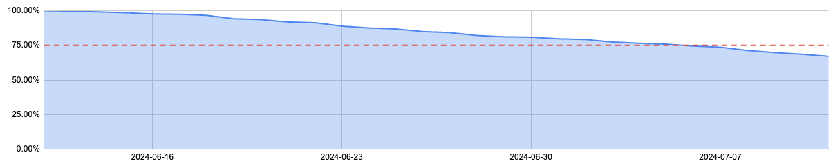
In this case, the error budget is the remaining 25% (100% - 75%). 25% is the maximum error rate the SLO can tolerate.
To track how much of the error budget is burned, the Y-axis of the reliability chart is scaled. In the example, 75% reliability corresponds to 0% of the error budget, while 100% reliability corresponds to 100% of the budget.
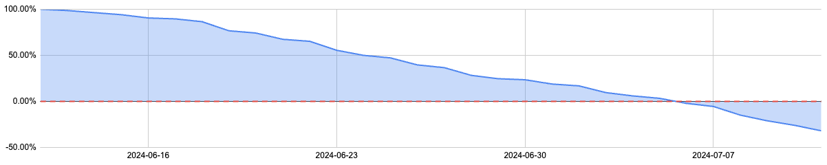
It's the same chart with different Y-axis labels. This representation clearly shows that the entire budget has been burned by the end of the visible time window, and it continues to burn beyond that. It falls below zero at the point where reliability falls below the target. When viewing the reliability chart, selecting a target for your standard SLO becomes straightforward.
Use cases
- Tracking HTTP requests (28-day rolling time window)
- A reliability target of 99.9% for such a service means that no fewer than 99.9% of all requests are successful within any 28-day period.
- Service availability (1-month calendar-aligned time window)
- A service is pinged every minute. It is expected to be available during a calendar month, with up to 1 hour of downtime allowance. This expectation translates to a reliability target of 99.86%.
30 days = 720 hours with a 1-hour error budget:
(720h–1h) divided by 720h gives 0.9986111 or 99.86% */}
- A service is pinged every minute. It is expected to be available during a calendar month, with up to 1 hour of downtime allowance. This expectation translates to a reliability target of 99.86%.
In composite SLOs, the reliability and error budget are tightly linked and assessed over the composite SLO's time window.
A composite SLO combines reliability or error budget states of its components. Particular calculations and the resulting representation depend on the component data consolidation and component weights.
Component weighing
Your complex system most likely includes services of different importance. For example, when you're monitoring the end-to-end user journey of your e-commerce store, errors when leaving a product review are pesky, but the payment service failures make users think twice about buying from this store. If you assign equal weights to these services, the less important ones would send redundant alerts, and the more crucial ones would dilute signals in the noise.
The higher the component weight, the greater its impact on the composite reliability.
When components have equal weights, the composite SLO considers their values directly, without additional processing.
With different weights, you can fine-tune the composite to reflect the importance of the components.
There's no limit to the absolute weight value. All component weights are normalized to 100% before being applied to the components to define their impact on the composite. The normalized weight is calculated using the following formula:
Component absolute weight / total absolute weights = component normalized weight
The weight proportion is the key—weights are determined by their relative values, not their absolute values. For example, weights of 2 and 4 are functionally equivalent to 50 and 100.
| Weight | Component A | Component B | Component C | Component D |
|---|---|---|---|---|
| Absolute, option I | 8 | 4 | 1 | 2 |
| Absolute, option II | 24 | 12 | 3 | 6 |
| Normalized | 53% | 27% | 7% | 13% |
Data consolidation
The point of composite SLOs is their ability to include a wide range of components. The data from these components must be consolidated to produce a single composite value.
You can select the aggregation metric to be applied to component data for consolidation. Two aggregation metrics are available:
- Reliability
- Error budget state
Aggregation by reliability
When component data is consolidated using the reliability metric, the per-minute composite reliability is calculated as follows:
- Calculate the per-minute reliability for each component (the ratio of successful events to total events for that minute).
- Apply user-defined weight to the reliability value of each component.
- Sum these weighted reliabilities and divide by the total of all component weights.
- Express the result as a percentage to get the per-minute composite reliability.
The examples provided below illustrate the impact of component weight on the composite reliability.
In a perfect world, if none of the components have any errors and report 100% reliability, the composite reliability is also 100%, regardless of component weight.
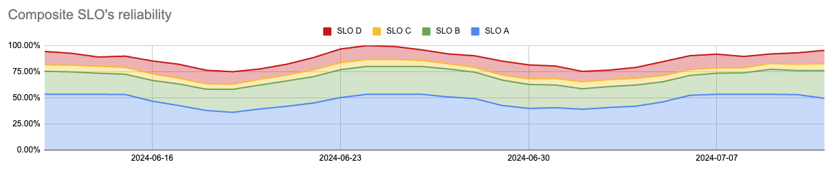
In real life, components do have some errors. So most often, their reliability falls below 100%. When all components have equal weights, the composite reliability only combines these values. Its reliability chart fluctuates, reflecting the plain sum of each component's reliability value.
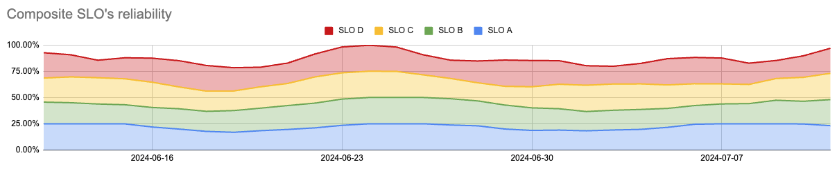
This "component stack" is presented as a single composite chart because component reliability values are normalized to 100%.
The reliability threshold of the composite SLO is visualized similarly to the standard SLO. Its error budget chart features a scaled Y-axis, and the reliability target is set to 0% of the error budget.
With equal weights, all components' contributions to the composite reliability are also equal. The weight factor is the way to fine-tune the components in the composite SLO. The component values are multiplied by their weights. The composite reliability changes depend now not only on the component values but also on their weights.
If none of the components have any errors, the reliability chart considers the components proportionally to their weights only:
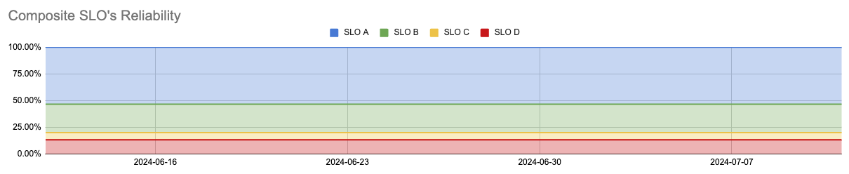
The impact ("thickness") of different component bands corresponds to their normalized weight.
Real-life SLOs rarely report stable 100% reliability. Component weights define their contribution to the composite reliability. The chart reflects the component values proportionally to their weights.
Aggregation by error budget state
The error budget state metric provides a high-level view of system health by evaluating whether components are "within" or "out" of the error budget, each minute.
- Assign a status to every component based on its remaining error budget at a specific point in time:
- 1 if the component has a positive remaining error budget.
- 0 if the component has completely burned its error budget.
- Apply user-defined weights to these binary values for each component.
- Sum these weighted values and divide by the total of all component weights.
- Express the result as a percentage to get the per-minute composite reliability.
When all components in a composite SLO have equal weights, the composite reliability is distributed evenly among them. The composite per-minute reliability is calculated by dividing the number of components that have positive error budget by the total number of components.
For example, a composite SLO includes four components—A, B, C, and D. On a given minute, Components B and C have a positive error budget. With equal weighting, the composite per-minute reliability is simply the sum of the normalized weights of components with positive error budgets:
25% + 25% = 50%
Assigning weights to the components accounts for their impact factor within the calculations.
The following example compares equal versus varied weighting for components reporting data over four minutes.
| Weight | Component A | Component B | Component C | Component D |
|---|---|---|---|---|
| Equal absolute weights | 3 | 3 | 3 | 3 |
| Equal normalized weights | 25% | 25% | 25% | 25% |
| Different absolute weights | 8 | 2 | 5 | 7 |
| Different normalized weights | 36% | 9% | 23% | 32% |
The composite per-minute reliability (the Result table columns) for the 4 one-minute periods is shown below, based on the error budget states of its four components:
| Minute | Component A | Component B | Component C | Component D | Result with equal weights | Result with different weights |
|---|---|---|---|---|---|---|
| 1 | 0 | 1 | 1 | 0 | 50% | 32% |
| 2 | 0 | 0 | 1 | 0 | 25% | 23% |
| 3 | 1 | 0 | 1 | 1 | 75% | 91% |
| 4 | 1 | 1 | 1 | 1 | 100% | 100% |
This effect is even more pronounced in minute 3. In the equal weight scenario, three positive components (A, C, and D) result in 75% per-minute reliability. But in the different weight scenario, the same three components contribute their specific normalized weights (36% + 23% + 32%), resulting in the composite per-minute reliability of 91%. This demonstrates that when a component with a higher weight (like Component A) has a positive budget, it contributes more significantly to composite reliability than a component with a lower weight.
- In aggregation by error budget status, all components look the same regardless of their complexity. Weighting ensures that a failure in a critical service has a proportional impact on the composite's reliability:
- If three minor services are healthy but the one critical database (Component A) is out of budget, an unweighted system would show 75% reliability.
- With different weights, that same failure in Component A could drop the composite reliability to 64% (as seen on Day 3 in the second fragment), signaling a much more severe issue.
Key takeaways
- Reliability is calculated as the ratio of successful events to total events or good minutes to total minutes over a specific time window.
- An error budget is the maximum number of bad events within a given time window a service can afford while remaining within its acceptable reliability level.
- The reliability target (e.g., 99.9%) acts as a threshold and impacts the error budget. If reliability falls below this target, then SLO's error budget is exhausted.
- Composite SLOs combine reliability or error budget state values from multiple underlying components into a single metric.
- The maximum portion of a composite SLO's reliability that can be burned by a single component equals to that component's normalized weight.
- Weights reflect the relative importance of various services (e.g., a payment service is usually weighted higher than a product review service).
- All absolute weights set by a user are normalized to 100% to define their relative impact on the composite reliability.
- Proper weighting prevents less important components from triggering redundant alerts or diluting signals from critical components.
- Weighting components ensures the composite reliability is mathematically anchored to components with the highest reliability targets, accurately reflecting critical component stability.
- Aggregation by error budget state uses a binary evaluation for each component. Binary values simplify complex telemetry into a clear, actionable signal.
- Aggregation by reliability uses the mean of weighted per-minute reliability values to determine the composite percentage.

