SLI Analyzer use cases
In this article, we will go over tree use cases of adjusting SLO targets using the SLI Analyzer for threshold and ratio metrics. Once we’ve adjusted our SLO targets, we can create a new SLO from our analysis.
Choosing the correct reliability target can be very challenging when it comes to establishing meaningful SLOs. There is no one-size-fits-all solution for good SLOs since reliability targets depend on how the system performed in the past.
SLI Analyzer can retrieve up to 30 days of historical data and lets you try out different reliability targets without creating a full-fledged SLO.
Tools to help you determine the desired reliability settings include the following:
- Statistical data displayed at the top of your analysis tab (e.g.,
Min,Max,StdDev). - The SLI values distribution chart that shows the frequency distribution of the data points in the given time window.
Understanding the historical performance of a service
Let’s assume that we’re an SRE responsible for our application's infrastructure, and we’d like to configure several SLOs on the service to ensure it meets reasonable response times targets.
To understand the historical performance of our system and pick relevant targets before creating SLOs, we used SLI Analyzer.
Go to the SLI Analyzer section on the Nobl9 Web. On the SLI analysis page, we select Datadog as a data source.
In these examples, we're using Datadog, but the overarching concepts are similar for all other observability platforms. In every example, we start with configuring data to be imported.
Use cases
- Analyzing latency (threshold)
- Analyzing successful server requests (ratio)
- Post-incident adjustment (threshold)
In this example, we're assessing the average response time made by the server to the client. For this, we analyze a Datadog threshold metric query.
Configure the analysis
We set a 14-day graph time window to calculate the error budget for two weeks.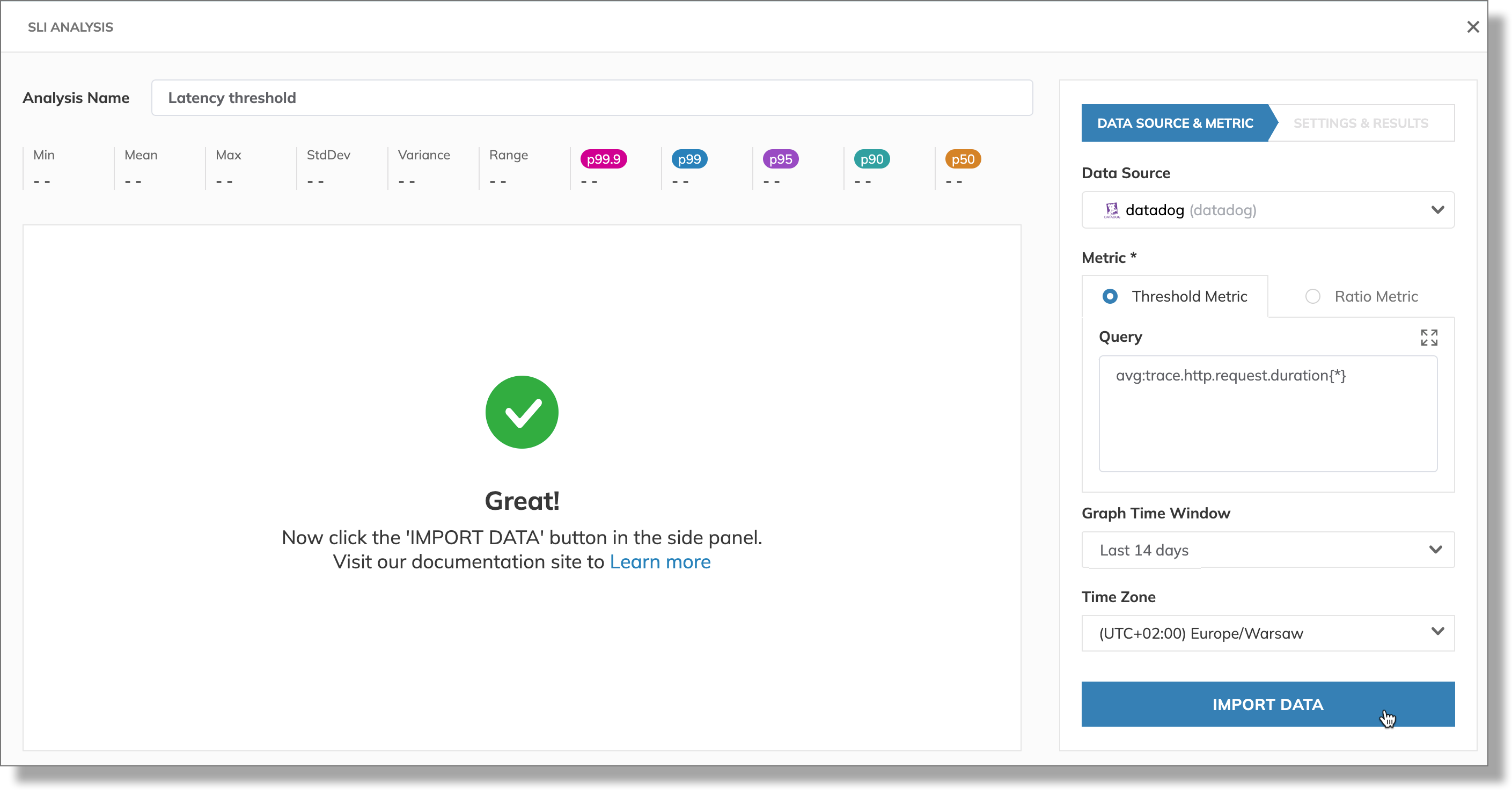
Assess raw data
After successful import, we can assess statistical data and percentile values. And view these values visualized in the charts: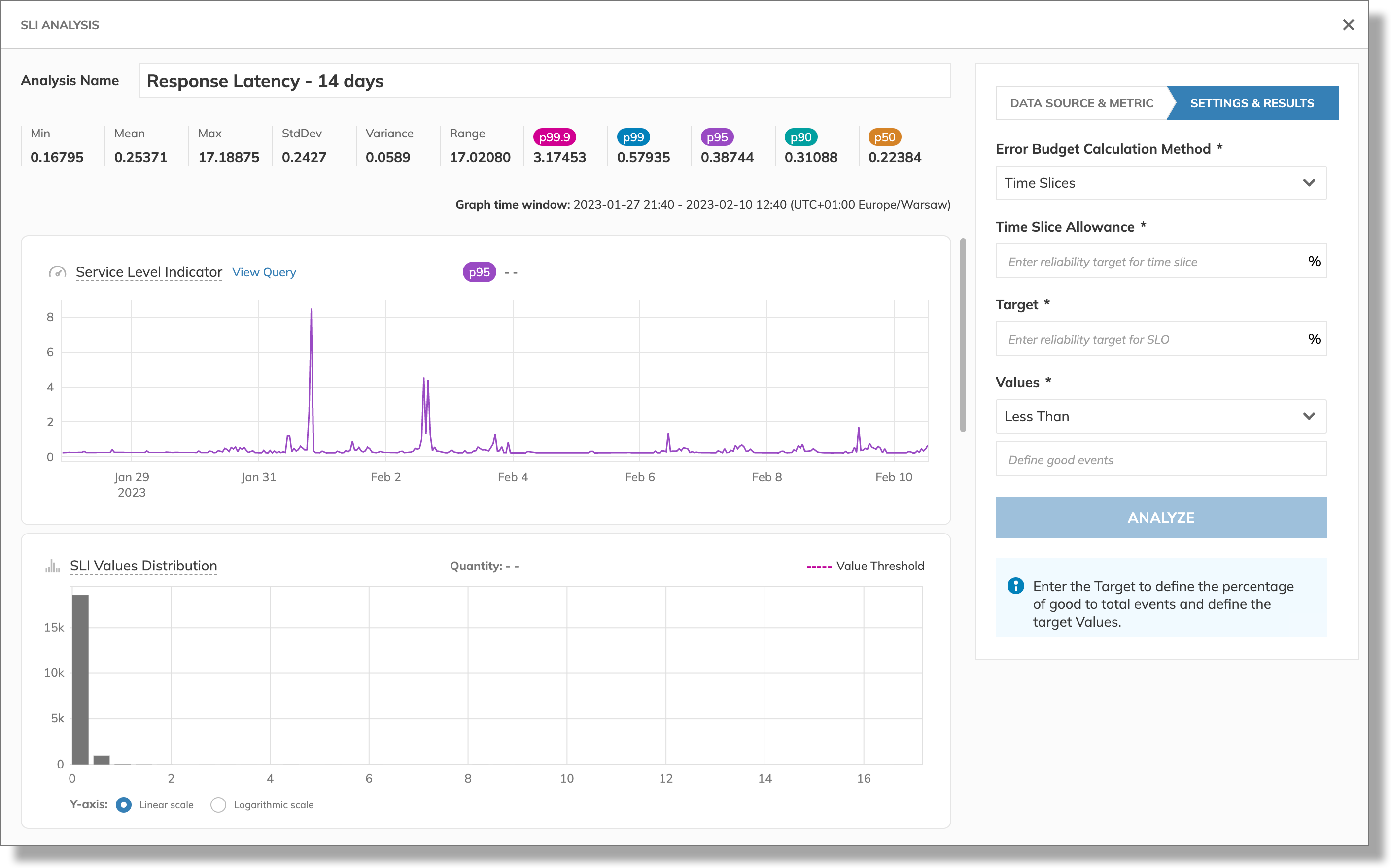
Since SLI value distribution is wide, we switch to the logarithmic scale to have more meaningful insight: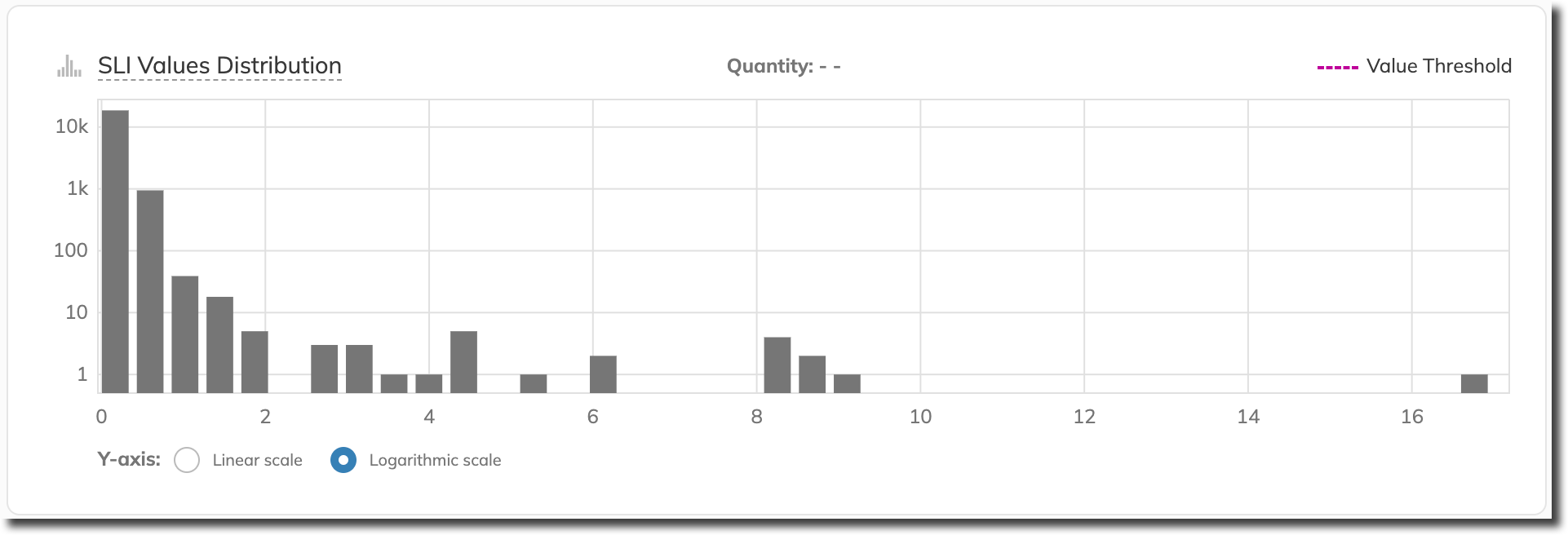
According to the statistical data, our application’s server sometimes responds quickly at around 0.16s—it's the Min value. At other times, it can take almost 17 seconds to send a response—the Max value: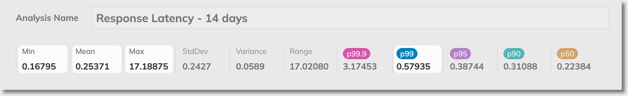
We can also note that their Mean value is around 0.25s—a reasonable average response time.
Next, we look at the percentile values and see that their p99 value is slightly below 0.6s.
Using the value of the 99th percentile,
we set the error budget calculation method to Occurrences with a threshold value of less than 0.6s: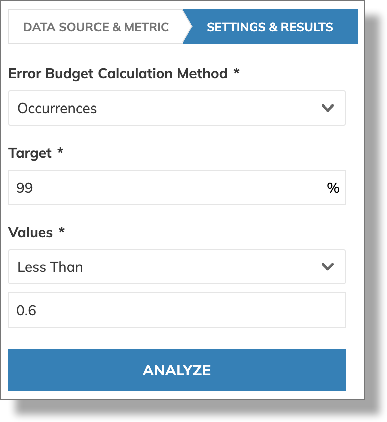
After analysis, we can see the Reliability burn down chart along with the analysis results: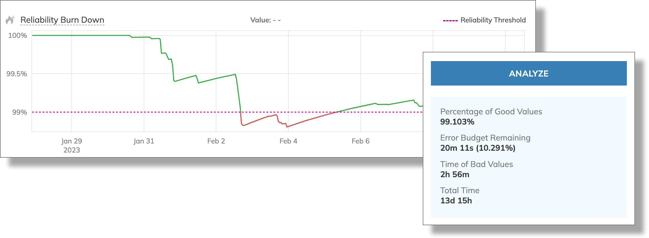
According to the analysis results, the percentage of good values is more than 99 (99.103%), and we have more than 10% of the error budget remaining (10.291%)
Adjust target
The SLI values distribution chart reveals that we can take into account only a portion of the values: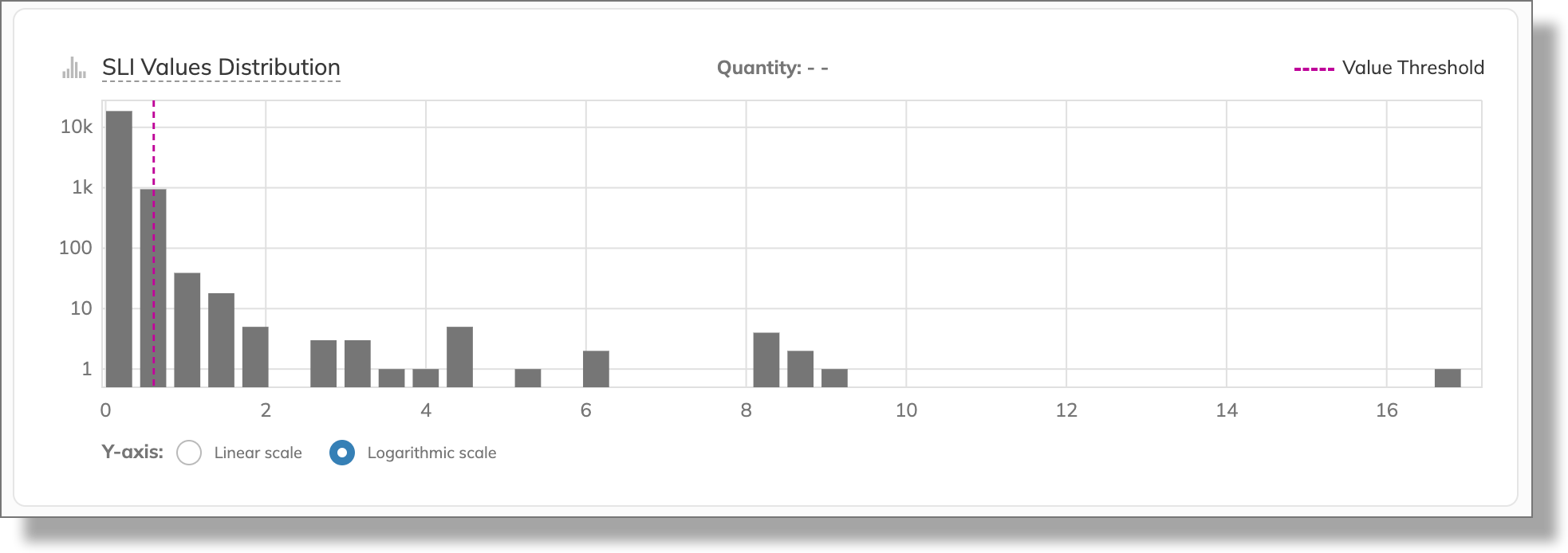
So, let's try a more strict threshold.
Changing the target value to 0.5 exhausts the error budget. Also, we’re slightly off the 99% target:
In conclusion, we consider 0.58s to be the acceptable value in the 99th percentile. Changing the values to be less than 0.58 allows us to stay within the error budget over the entire 14-day time window: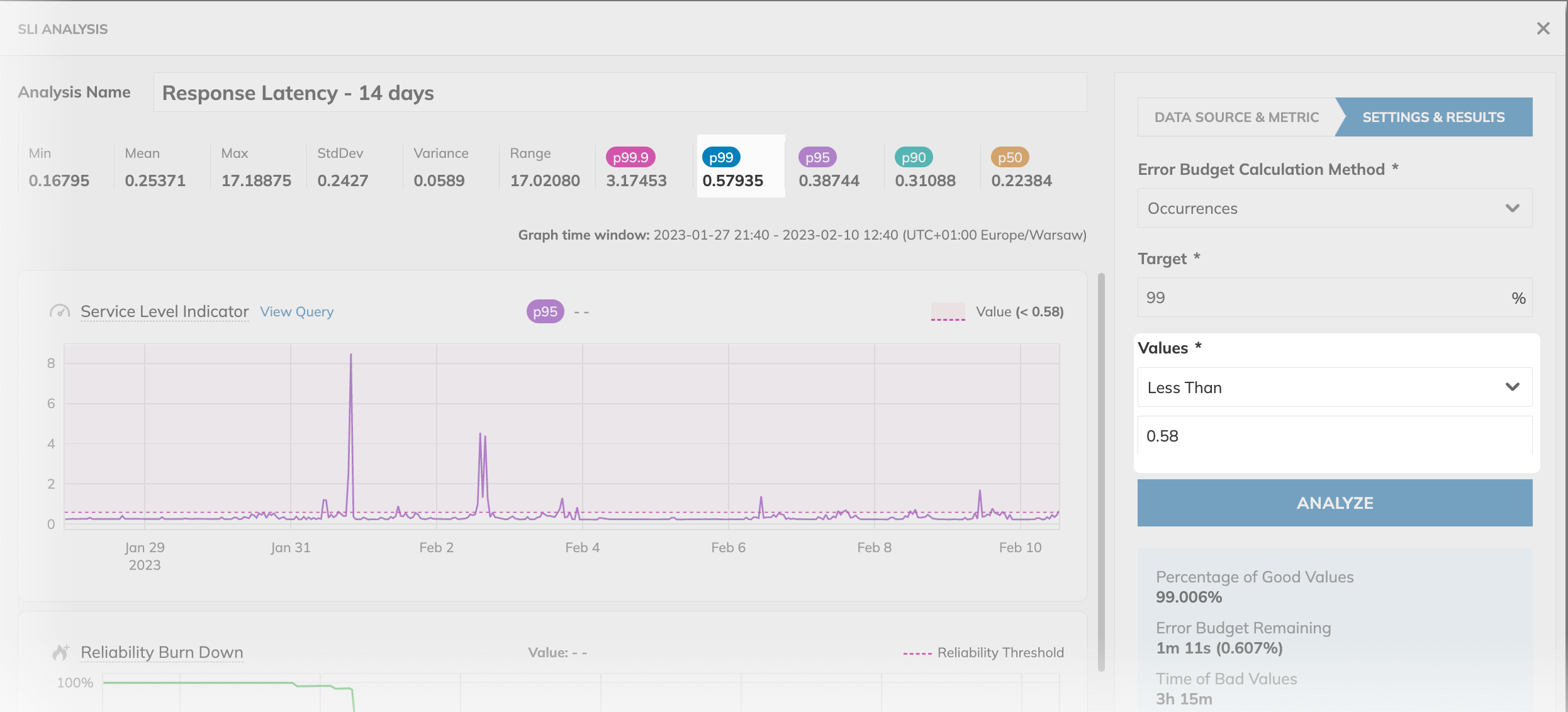
With SLI Analyzer, we can try different reliability targets for the ratio metrics.
In this example, we're accessing successful server requests (HTTP status code in the 2xx and 3xx ranges) for our application instance.
Configure the analysis
We use a 24-hour graph time window to scrutinize the performance of our application over one day.
Once the data import is complete, we can see statistical values and the charts for the good and total metric values we selected: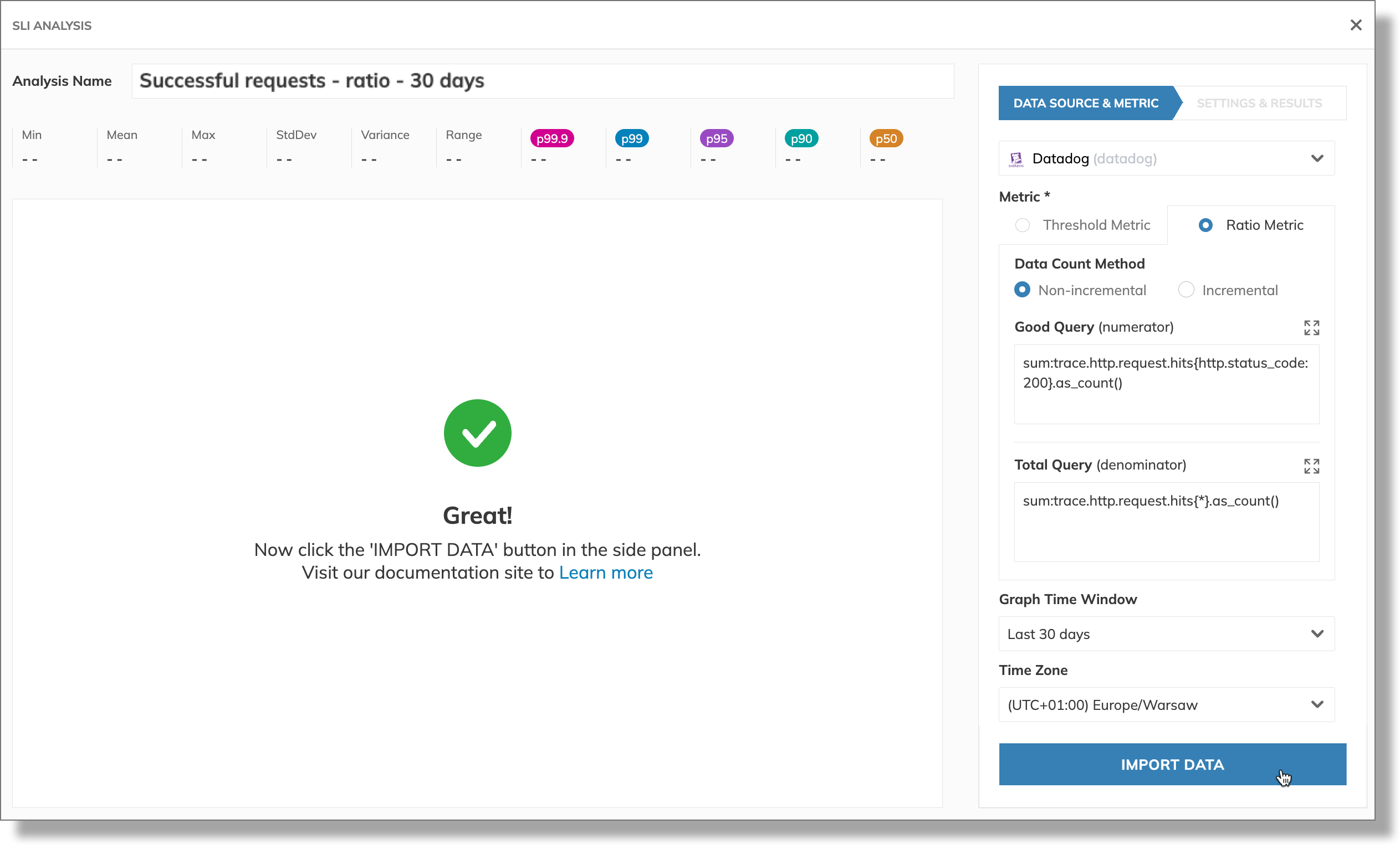
Once data is imported, we can try different configuration for the SLO. For this, we set the Target value to 95 and run the analysis to evaluate the error budget against it. Our analysis indicates that the current good value percentage of 95.72% would result in a tiny error budget excess—almost 10 minutes: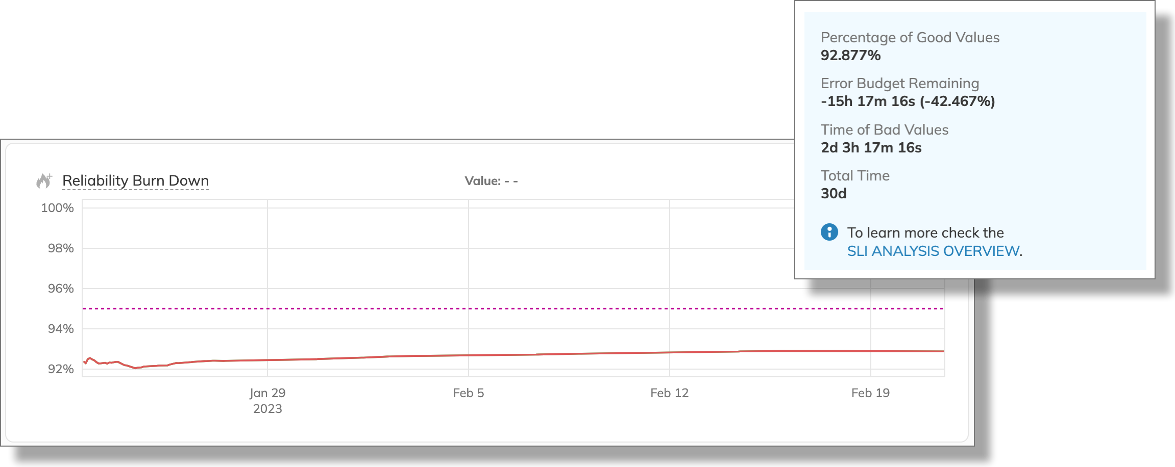
Adjust target
We consider acceptable to reach 90% good events for our application server. So, we adjust the target to 90% for the same window to re-evaluate the error budget. We run the analysis again, with the new target: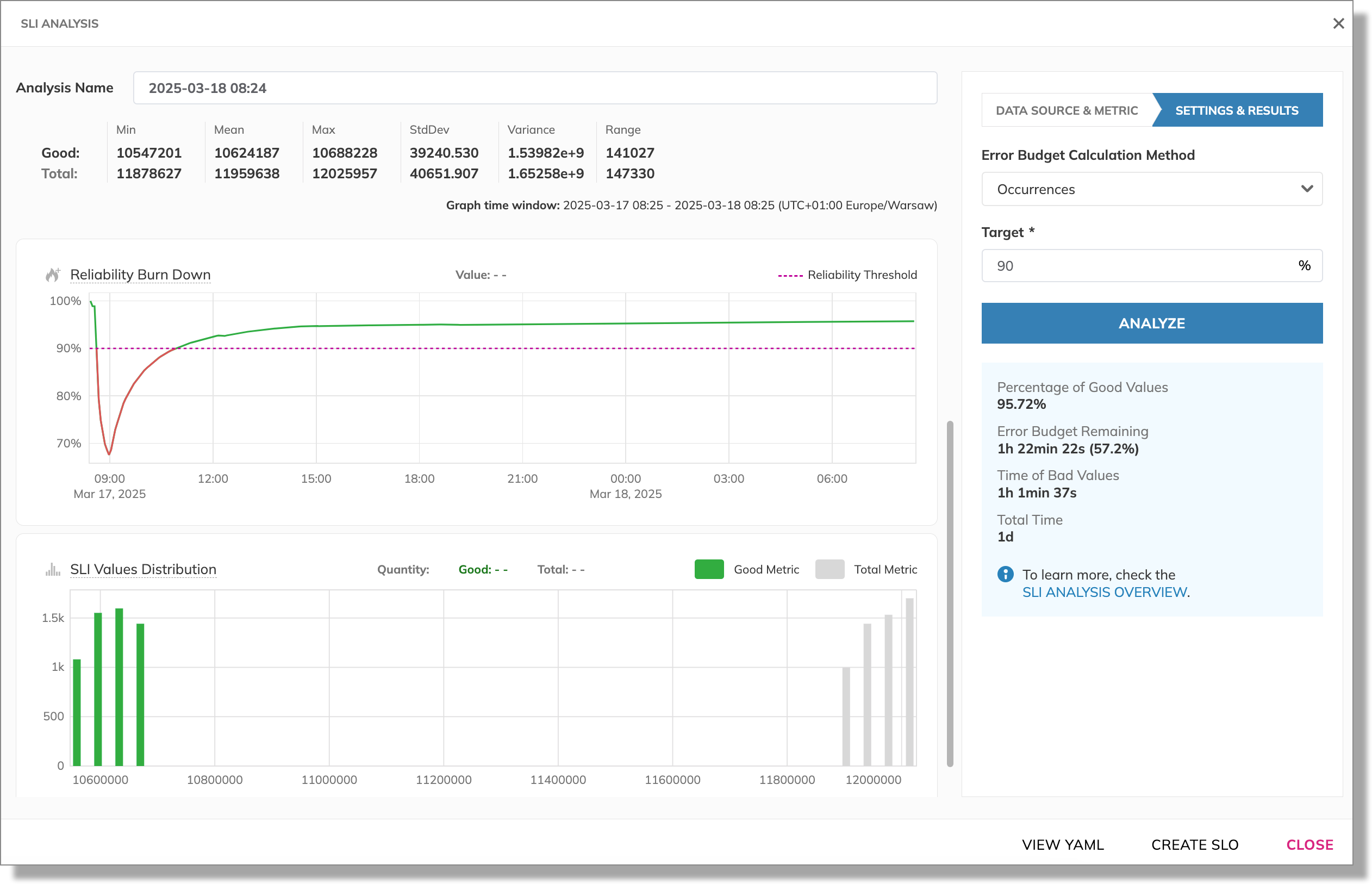
With this target, our SLO reaches the “green” zone—it reports the remaining error budget of almost one hour and a half.
SLI Analyzer can also be helpful when conducting post-incident analyses on your SLOs after incidents and allows you to readjust your SLO’s targets and thresholds.
In this example, we analyze a threshold metric from when the system had an incident. We examine the values for our SLO over the last 30 days to learn the performance trends before the incident and see how the incident affected the error budget.
Once the data is imported, we can examine the statistical values: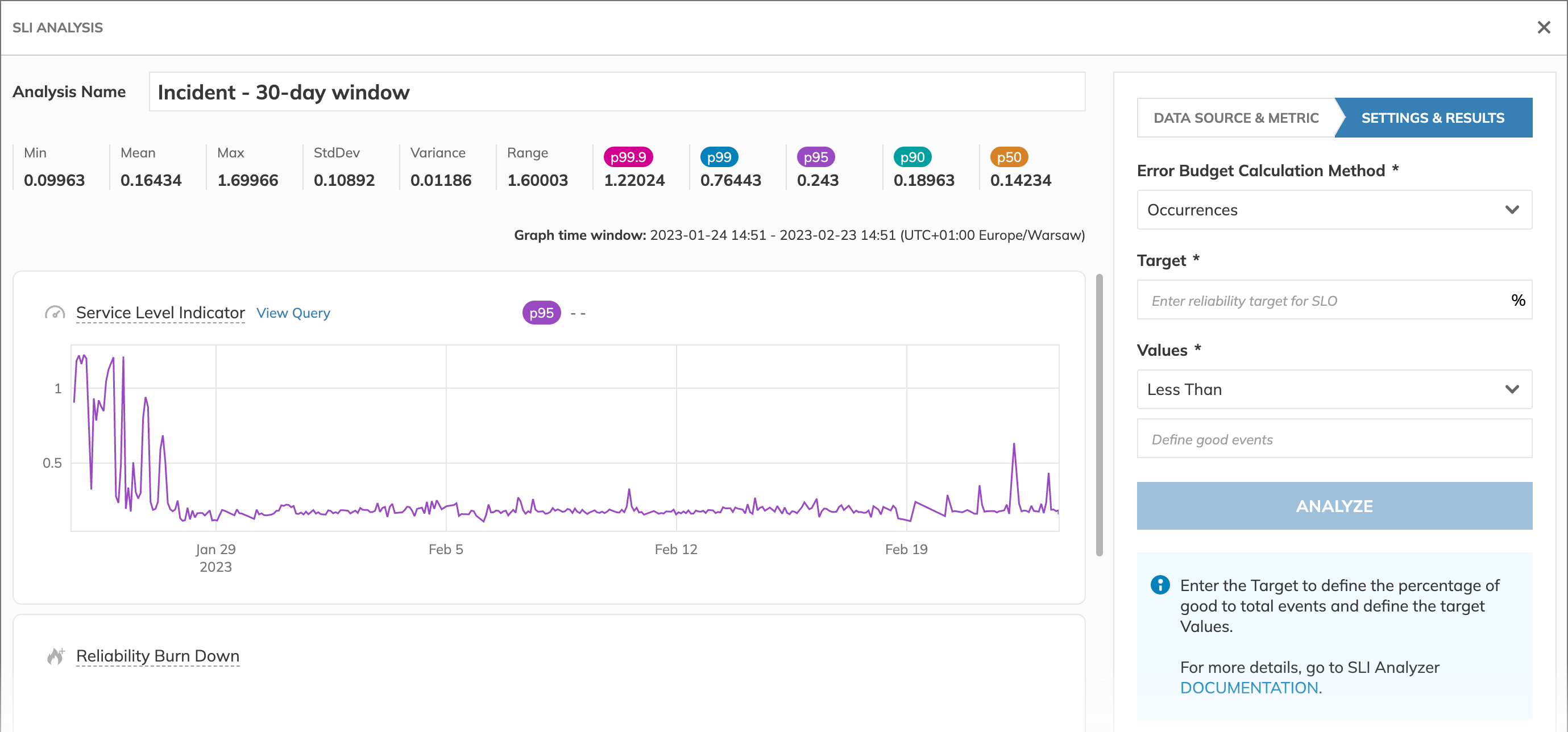
Evaluate the error budget with 99% of the values in the distribution to be below the 95th percentile: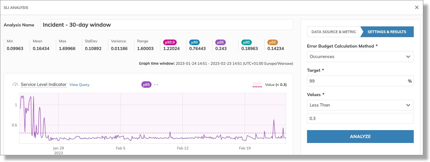
After the analysis, we see the major setback in the reliability and the severe error budget overrun: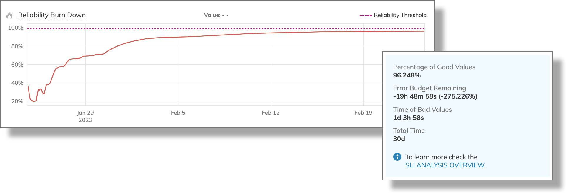
The logarithmic scale displays a long tail of aggregated high latency values: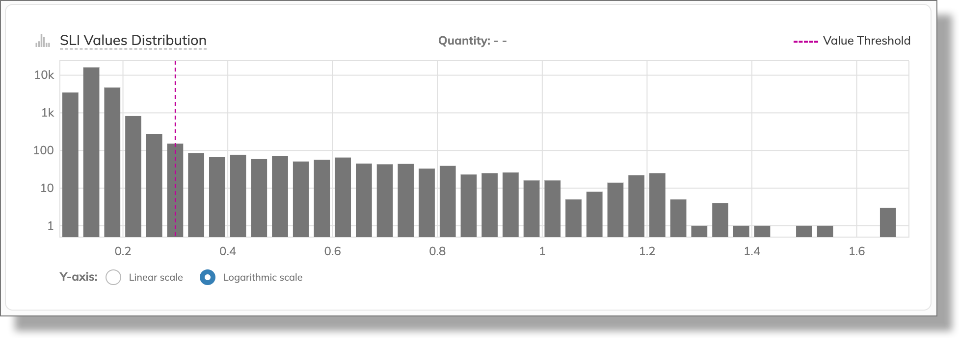
We can now estimate the impact of the incident. Even with a generous margin for values, our reliability burn is red. We end up with almost -20 hours of the error budget, and the total time of bad values is more than one day.
The analysis revealed that an external server triggered the incident. This was an isolated occurrence with a low probability of repetition. So, we excluded the incident from the investigation for our second attempt by reducing the graph time window to 14 days. This will help us determine if we can recover our error budget.
For this, we need to create a new analysis to assess SLI data over a different time window with the same query.
This time, we set the Last 14 days for the graph time window. Imported data appears as follows: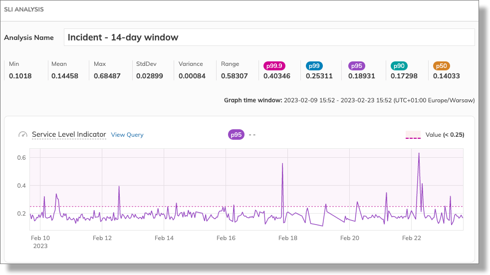
Before adjusting the target, observe the statistical data and the SLI chart.
| Value | 30-day GTW | 14-day GTW |
|---|---|---|
Mean | 16ms | 14ms |
Max | 1.69s | 68ms |
p99 | 0.76s | 0.25s |
The comparison between the 30-day and 14-day graph time window shows little changes in the mean value, while the maximum value increased significantly. Similarly to the maximum value, the 99th percentile changed: it's three times lower when the incident isn't taken into account.
Analyzing the SLI with a bit higher 99th percentile value, 0.26, we observe that excluding the incident regains the entire error budget. As a result, we have a healthy margin of 28 min 30 s—14% of the error budget.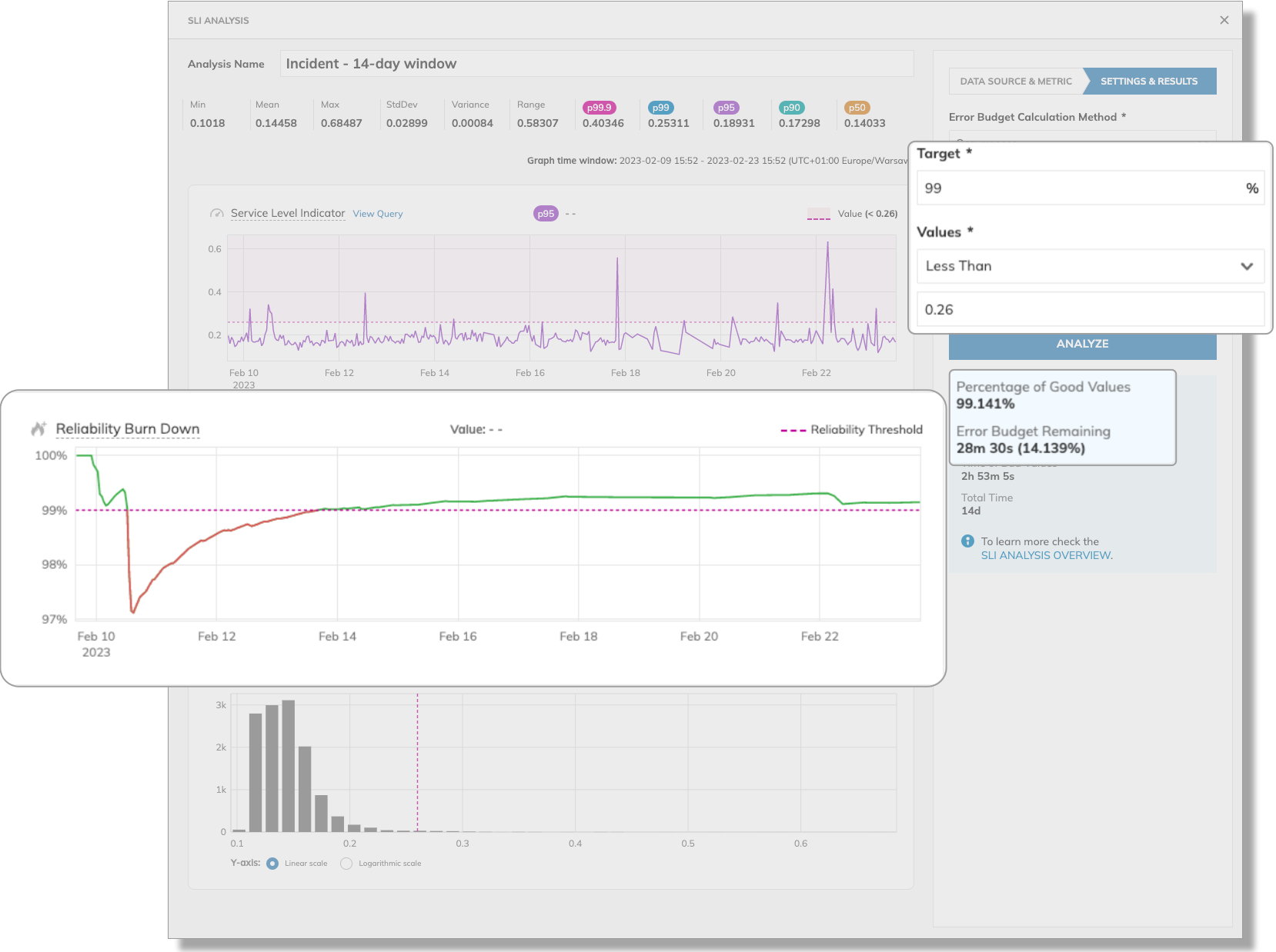
Happy with the outcome, we go ahead and create a new SLO from our analysis.
Query and SLO reference
In our examples, we used the following queries:
- Latency analysis:
avg:trace.http.request.duration{*} - Successful request analysis:
- Good query
sum(my-application_server_requests{code=~"2xx|3xx",host="*",instance="XXX.XXX.XX.XXX:XXXX"}) - Total query
my-application_server_requests{code="total",host="*",instance="XXX.XXX.XX.XXX:XXXX"}
- Good query
- Post-incident analysis:
avg:trace.http.request.duration{*}

