Explore real-world SLOs
- Pod readiness transition: threshold
- API server response latency: ratio
Let's create an SLO to monitor the stability of pod readiness transitions over a specific time period. To achieve this, we need to track how often pods in our Kubernetes cluster transition between "ready" and "not ready" states within the past 5 minutes.
In this case, we are monitoring readiness transitions, which behave monotonically. The total number of transitions either increases or remains the same during a given time window, as each state change is counted incrementally. This counter resets only when a new monitoring time window begins. Considering these characteristics, we’ve selected the threshold metric type.
To put this into practice, we can use the following PromQL query to measure state changes in pod readiness:
sum(changes(kube_pod_status_ready{condition="true"}[5m]))
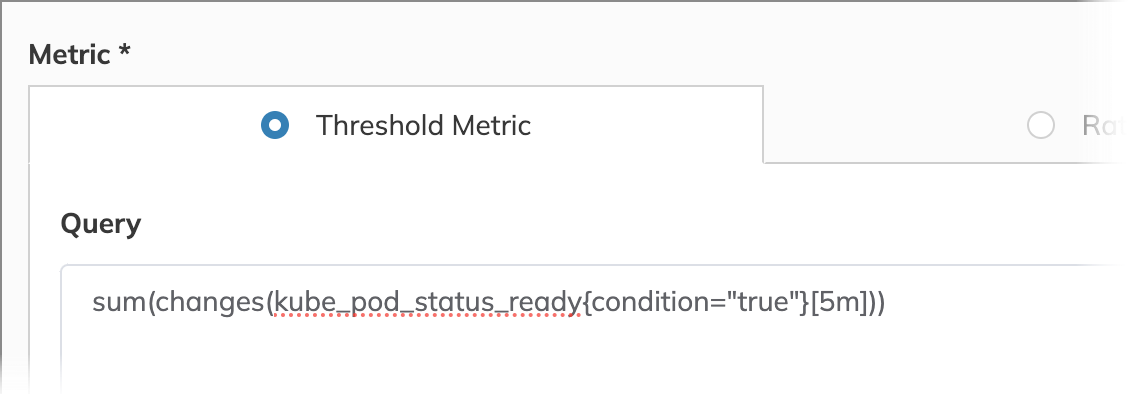
Looking for an alternative metric type? Check out the ratio metric type, designed to compare good responses to total responses.
The rolling time window is ideal here because it allows for continuously updating metrics in real-time. In this scenario, we’re focusing on a week-long view, setting the time window duration to seven days. This means our error budget will be calculated dynamically across this period, continuously incorporating fresh data as older points are replaced.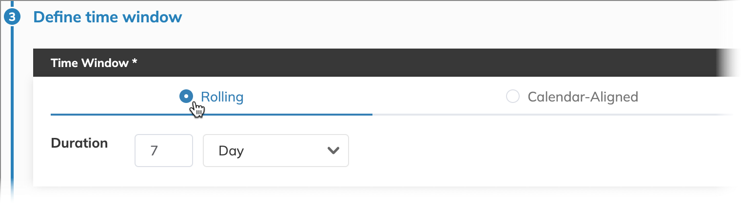
Curious about alternative time windows? Explore the benefits of calendar-aligned time windows for your use case.
To track and control the frequency of readiness state changes, we use the occurrences error budget calculation method. With this budgeting method, we monitor how frequently state changes occur within 5-minute intervals (set in the query).
While normal operation allows for some state transitions, we assume that our error budget is depleted when 7 or more state transitions occur in a single 5-minute interval, as this frequency may indicate underlying pod stability issues. This target, combined with a 99.5% success rate, ensures we maintain both reliability and stability.
For clarity, we name this SLO objective Acceptable readiness transitions. In this example, it is the only objective in our SLO.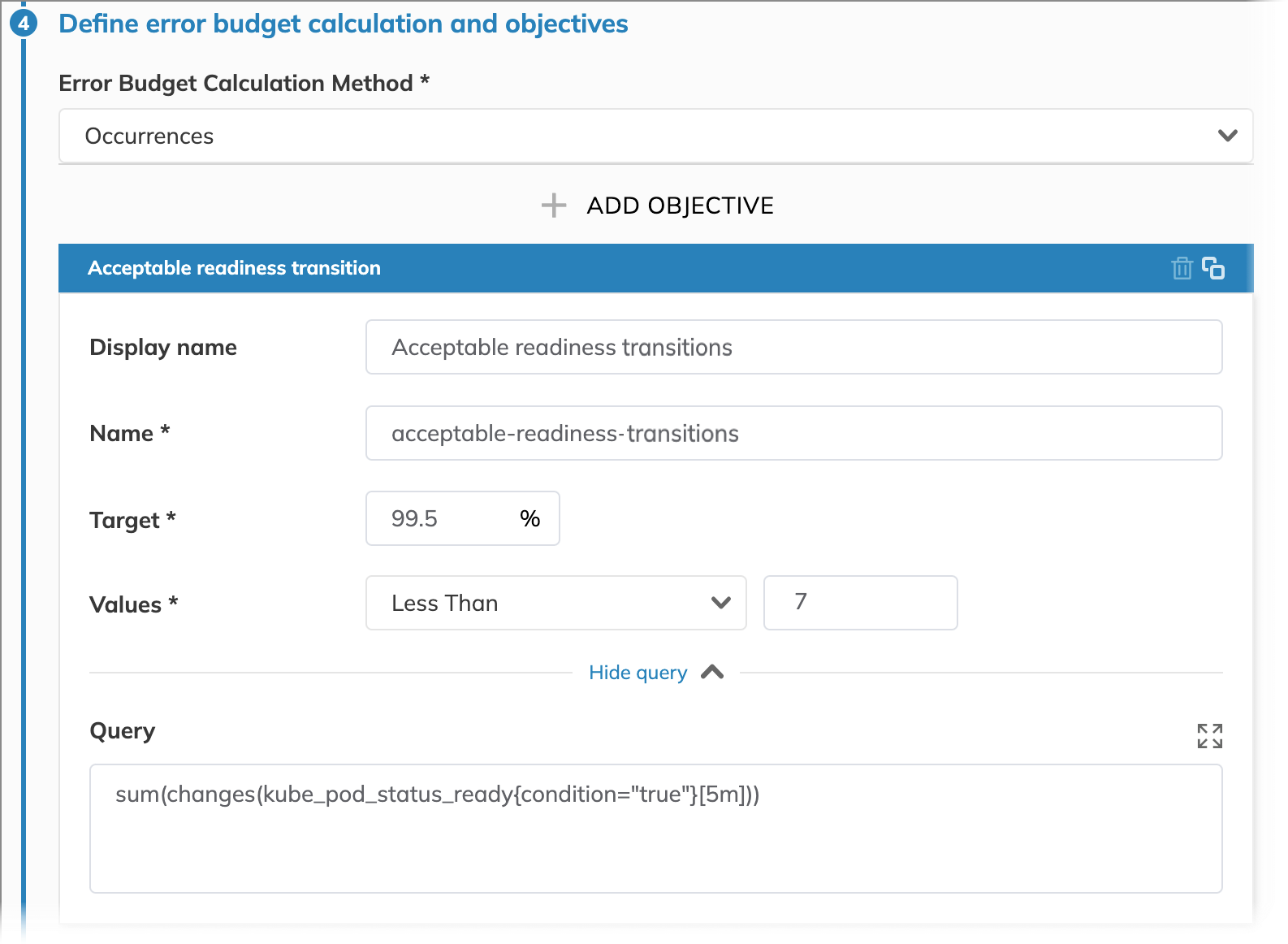
Interested in alternative methods? Explore the timeslices error budget method.
The final step is to make the SLO user-friendly and easy to collaborate on. This includes giving it a clear name and applying optional settings for streamlined management.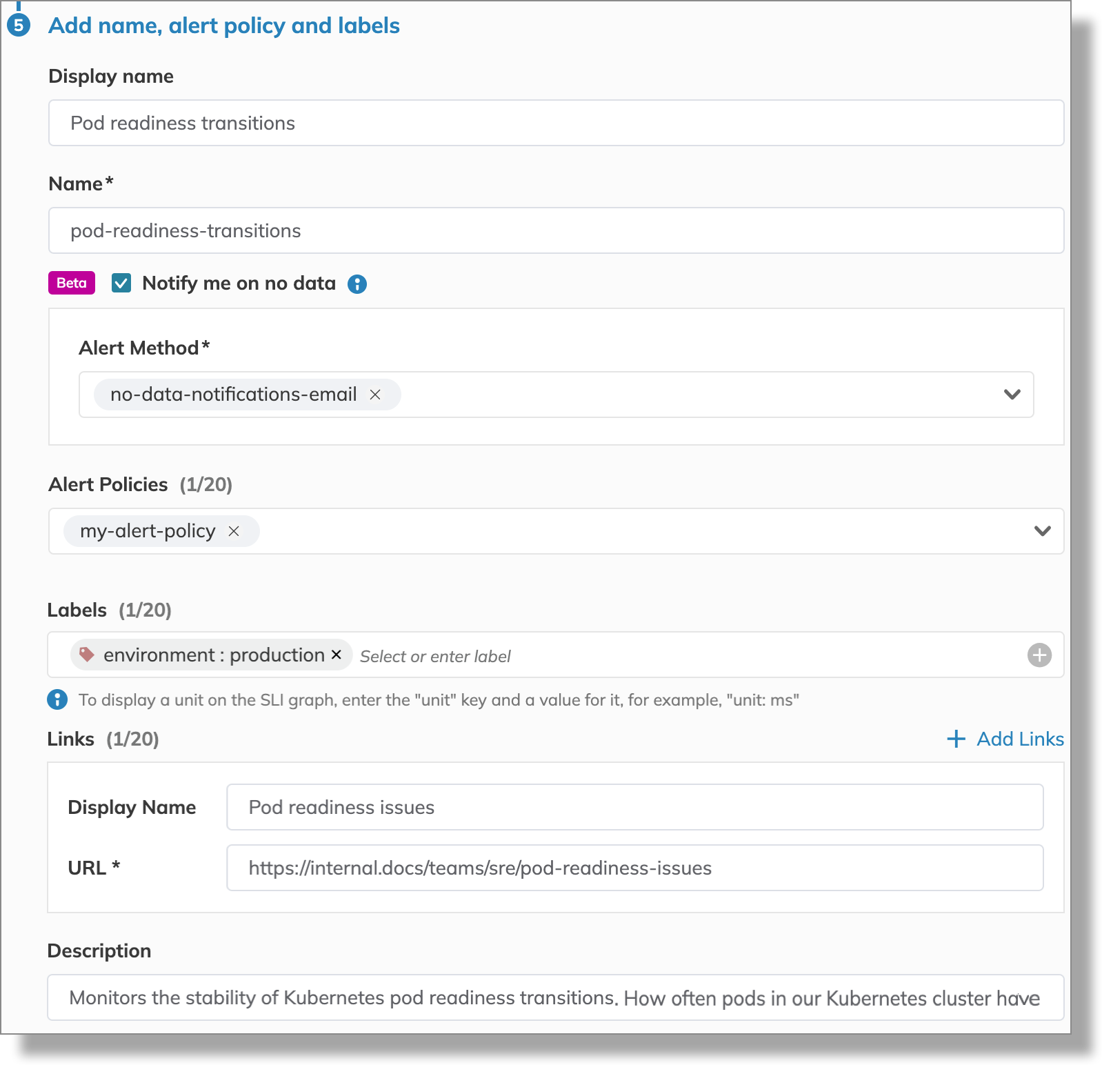
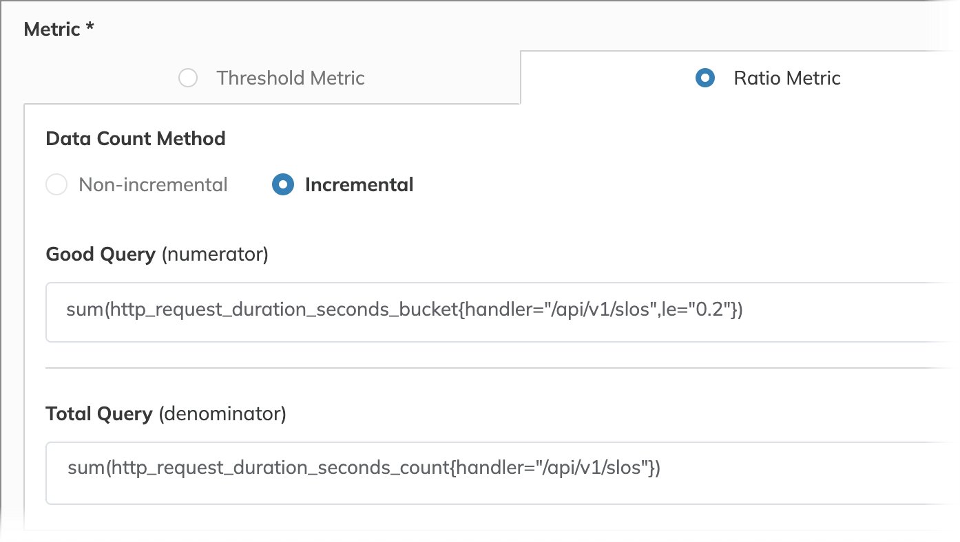
Let's create an SLO to monitor the time it takes for our API server to respond. For this, we want to compare the number of low-latency responses to the total number of responses over a specified time frame. We define a "good" response as one completed in 200 milliseconds or less.
Response latency can vary unpredictably within the same time window due to factors like changes in server load, network conditions, or fluctuating request volumes. To account for this variability and track performance, we use the ratio metric type, comparing low-latency responses to total responses.
We select the incremental data count method because it tracks the cumulative count of responses over the time window, allowing us to evaluate performance in real time.
To configure these metrics in our monitoring system, we use the following PromQL queries:
Good: sum(http_request_duration_seconds_bucket{handler="/api/v1/slos",le="0.2"})
Total: sum(http_request_duration_seconds_count{handler="/api/v1/slos"})
Want to explore other metric types? Check out the threshold metric type, which focuses on raw metrics rather than ratios.
We aim to evaluate our API server's performance weekly to ensure a balance between capturing overall trends and allowing sufficient time for remediation, without being overly sensitive to transient fluctuations. Thus, a calendar-aligned time window of one week is appropriate.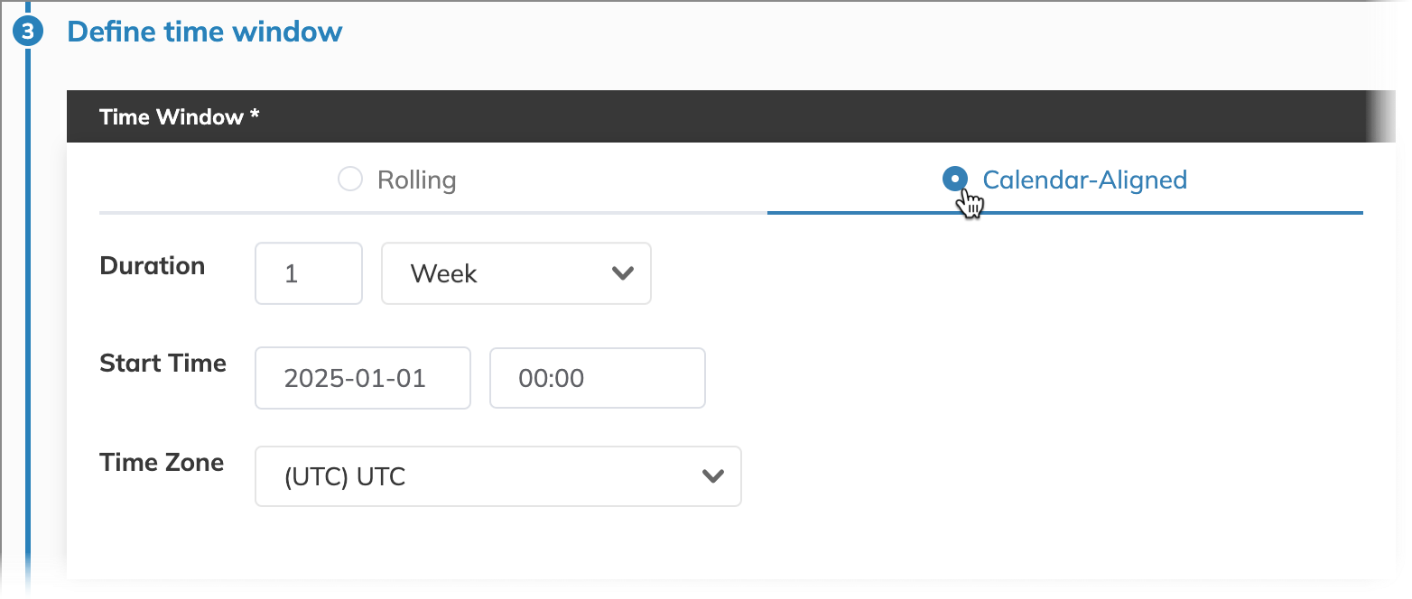
Curious about alternatives? Learn about rolling time windows, which offer a continuously shifting view of performance.
We accept our API server exceeding its expected latency for up to 5% of the time per week. We chose the timeslices error budget calculation method because it provides a minute-by-minute analysis of performance. We consider a minute good if 90% of data points obtained during this minute will indicate the latency of 200 milliseconds or less. The target of 95% means we expect at least 95% of all minutes within a week to be good minutes.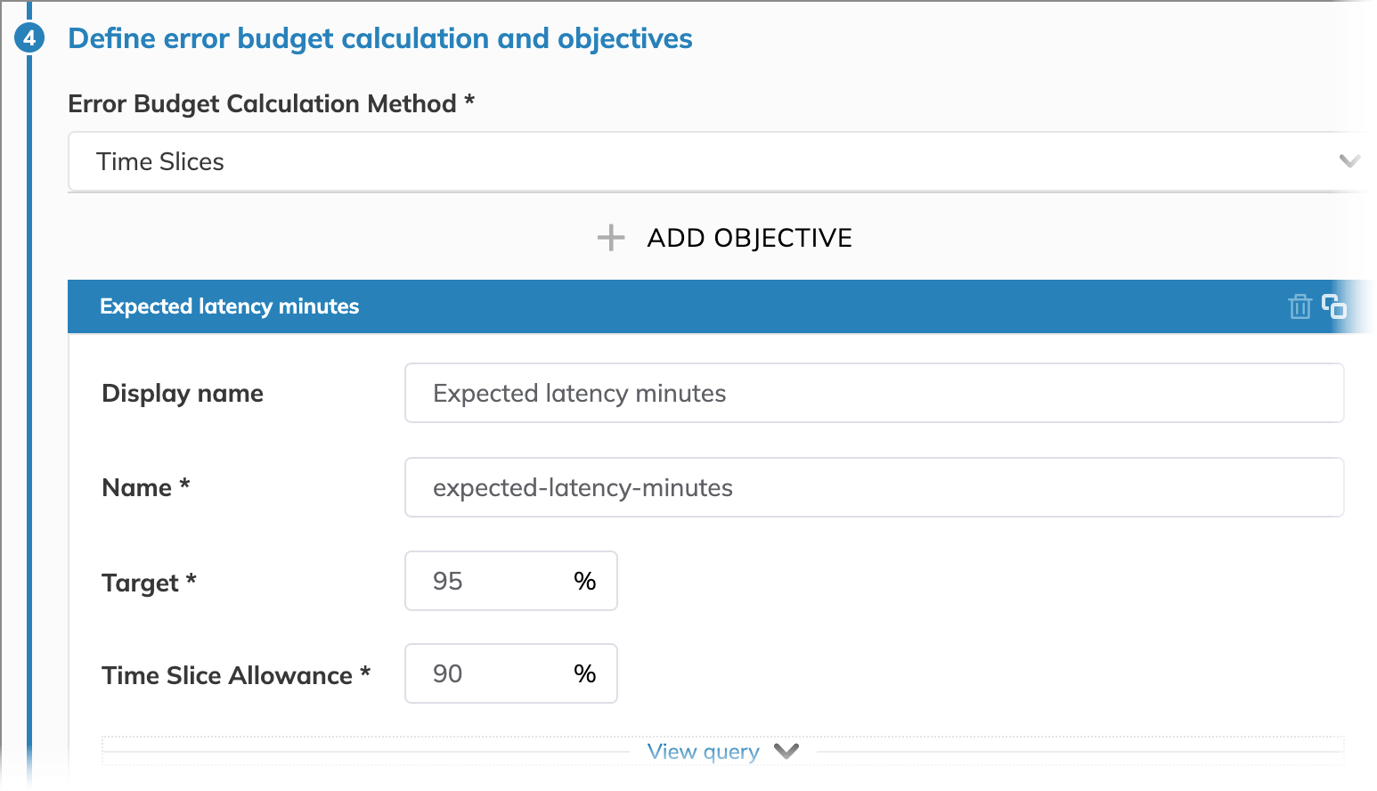
Interested in other approaches? Explore the occurrences error budget calculation method for tracking threshold metrics.
The final step is to make the SLO user-friendly and easy to collaborate on. This includes giving it a clear name and applying optional settings for streamlined management.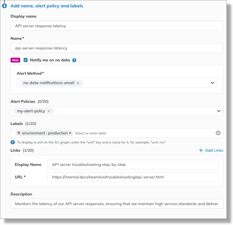
- As you're typing a display name for your Nobl9 resource (here—the SLO and its objective), Nobl9 automatically generates the name for it.
nameis a unique identifier for all resources in Nobl9. You can manually set it only once, when creating a resource. After you save your resource, the name becomes read-only. You will need your resource name when working withsloctlto specify the names of required resources in a YAML definition.